12.9 Computing pairwise distance

Read in the FASTA file of aligned sequences with the read.dna function from ape:

dna <- read.dna("aligned.fa", format = "fasta", as.matrix = TRUE)

We then compute the pairwise distance matrix:

D <- dist.dna(dna, model = "TN93", as.matrix = TRUE)

We can plot this matrix to visualize it:

# use the "melt_dist" function from harrietr package to convert
# the distance matrix to "long" format for ggplot
D_melted <- rbind(melt_dist(D, order = ids),
                  melt_dist(t(D), order = rev(ids)))

# plot distance matrix
ggplot(data = D_melted) +
  geom_tile(aes(x = iso1, y = iso2, fill = (dist + 1e-5))) +
  theme_classic() +
  theme(axis.text.x = element_text(angle = 90, hjust = 1)) +
  scale_fill_viridis_c(name = "distance") +
  xlab("sample") +
  ylab("sample")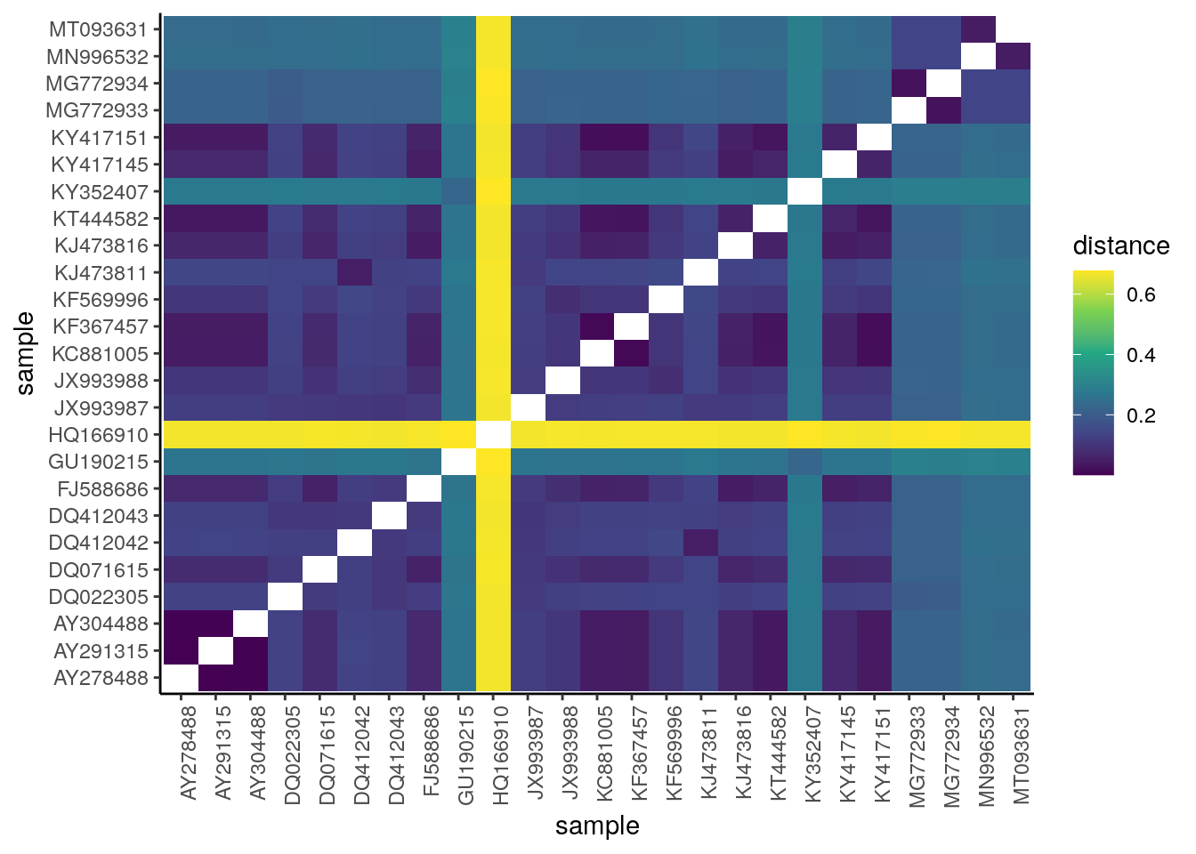

Interpreting the distance matrix

Most of these coronaviruses seem to be fairly similar – i.e., there’s no clear clustering of sequences – besides HQ166910, which looks genetically distinct from the other sequences.