6.20 Required homework

Assignment: Re-run the steps we used to generate our PCA plot, this time using the all dataframe. Do these plots look any different from our plots with just common variants?

Solution

# extract genotypes and convert to matrix
gt_matrix_all <- all[, 7:2510] %>%
  as.matrix()

# transpose
gt_matrix_T_all <- t(gt_matrix_all)
# perform PCA
pca_all <- prcomp(gt_matrix_T_all)

# extract coordinates from PCA object
x_all <- pca_all$x

# create dataframe for plotting
pca_results_all <- data.frame(sample = rownames(x_all),
                              PC1 = x_all[, 1],
                              PC2 = x_all[, 2],
                              PC3 = x_all[, 3])
# merge with metadata
pca_results_all <- merge(pca_results_all, metadata,
                         # specify columns to merge on
                         by.x = "sample", by.y = "sample")

# calculate variance explained by each PC
var_explained_all <- pca_all$sdev^2 / sum(pca_all$sdev^2)
# print for PC1-PC3
var_explained_all[1:3]

## [1] 0.09154081 0.03824824 0.01207284

# PC1 vs. PC2 plot
ggplot(data = pca_results_all, 
       aes(x = PC1, y = PC2, color = superpop)) + 
  geom_point() + 
  xlab("PC1 (9.15%)") +
  ylab("PC2 (3.82%)")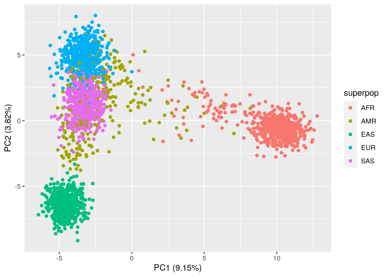

# PC2 vs. PC3 plot
ggplot(data = pca_results_all, 
       aes(x = PC2, y = PC3, color = superpop)) + 
  geom_point() + 
  xlab("PC2 (3.82%)") +
  ylab("PC3 (1.21%)")

The PCA plots actually look pretty similar to the plots with just common variants!