6.21 Optional homework

We can think of our PCA as a model of human individuals. If we have a mystery individual but we know their genotypes for the variants in our PCA, we can predict where they should lie in PCA space and thus guess their ancestry.

We’ve prepared a file, unknown.txt, which contains genotypes for one mystery sample (NA21121). We’ll compare it to the PCA model that you created for the required homework.

Follow the instructions to predict NA21121’s placement on your PCA plot.

6.21.0.1 Prepare unknown sample for PCA

Assignment: Read in unknown.txt, convert it to a matrix, and transpose.

Solution

# read VCF
unknown <- read.table("unknown.txt") %>%
  as.matrix()

# transpose matrix
unknown_T <- t(unknown)

6.21.0.2 Predict PCA placement of unknown sample

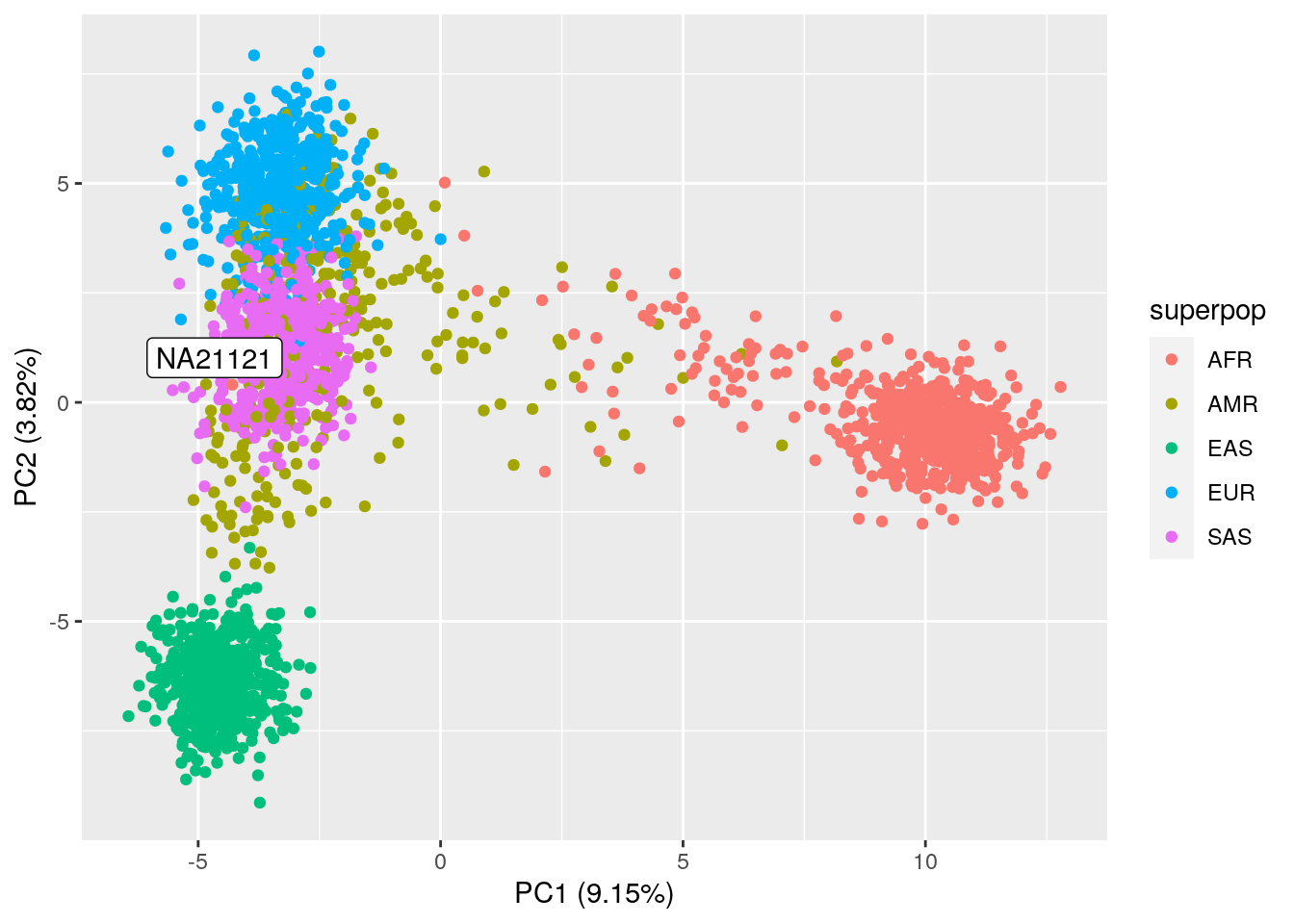
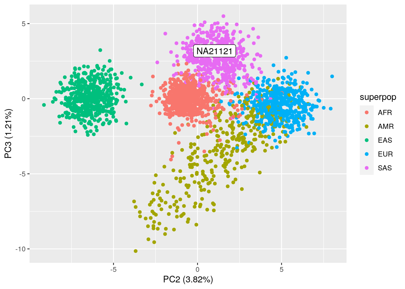
Assignment: Run the code block below to predict and plot NA21121 on top of your PCA plot from the required homework. If necessary, plot PC2 vs. PC3 as well. What superpopulation do you think NA21121 is from?

Solution

# predict pca placement of unknown data
unknown_pca <- predict(pca_all,
                       unknown_T)

# create dataframe from predicted PCA
unknown_results <- data.frame("PC1" = unknown_pca[, "PC1"],
                              "PC2" = unknown_pca[, "PC2"],
                              "PC3" = unknown_pca[, "PC3"],
                              "sample" = "NA21121")

# plot PC1 vs. PC2 and then predicted sample
ggplot() +
  # PCA plot from required homework
  geom_point(data = pca_results_all, 
             aes(x = PC1, y = PC2, color = superpop)) +
  # plots the unknown sample's location on the PCs
  geom_label(data = unknown_results,
             aes(x = PC1, y = PC2, label = sample)) + 
  xlab("PC1 (9.15%)") +
  ylab("PC2 (3.82%)")

# plot PC2 vs. PC3
ggplot() +
  geom_point(data = pca_results_all, 
             aes(x = PC2, y = PC3, color = superpop)) +
  geom_label(data = unknown_results,
             aes(x = PC2, y = PC3, label = sample)) + 
  xlab("PC2 (3.82%)") +
  ylab("PC3 (1.21%)")

NA21121 seems to be part of the SAS (South Asian) superpopulation. If we look up the sample ID in the 1000 Genomes database, we can confirm that it’s part of the Gujarati Indians in Houston, TX.