2.7 Navigating IGV

Once you’ve clicked on a chromosome, zoom in until you can see colors on the top track. This track displays the DNA sequence, colored by nucleotide.

The track below the DNA sequence has gene annotations from RefSeq.

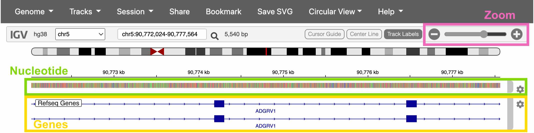
Fig. 12. Viewing a gene in IGV.

---

All illustrations CC-BY.
All other materials CC-BY unless noted otherwise.