5.21 Homework

One way to extend our simple Wright-Fisher model is to add in selection as a parameter. Selection affects our model by altering the probability of sampling our allele of interest each generation (e.g., positive selection increases the probability, and negative selection decreases it).

Previously, we assumed that this probability was equivalent to the allele’s frequency, or \(p = \frac{i}{N_e}\), where \(N_e\) is the population size and \(i\) is the number of individuals who carry the allele.

For the purposes of this homework, we assume that in a model with selection, this probability is instead:

\[ p = \frac{i(1 + s)}{N_e - i + i(1+s)} \]

where \(s\) is the selection coefficient, and ranges from -1 to 1.

What does this probability become in the absence of selection (i.e., when \(s = 0\))?

The probability becomes \(\frac{i}{N_e}\), which is the same as the allele frequency.

5.21.0.1 Learning Objectives

Practice writing functions in R
Interpret allele frequency trajectories under selection and drift

5.21.0.2 Assignment

In the code block below, modify your run_sim function so that it takes in a selection coefficient s as a parameter. Run the simulation a few times with and without (s = 0) selection, but keeping other parameters the same (Ne = 10000, freq = 0.5, generations = 10000). What do you notice about the allele frequency trajectories?

Note that most selection coefficients are thought to be extremely small – the largest known selection coefficients in humans are around 0.05.

Solution

# simulation function with selection
run_sim_selection <- function(Ne, freq, generations, s) {
  
  freq_vector <- freq
  for (i in 1:generations) {
    # calculate p, the probability of sampling the allele, based on s
    i <- freq * Ne # number of individuals who currently carry the allele
    p <- i*(1+s) / (Ne - i + i*(1+s))
    
    # prob is now `p`, rather than `freq`
    new_freq <- rbinom(n = 1, size = Ne, prob = p) / Ne
    freq_vector <- c(freq_vector, new_freq)
    freq <- new_freq
  }
  
  # convert vector of AFs into a tibble for plotting
  sim_results <- tibble(afs = freq_vector,
                        gen = 1:(generations+1))
  
  # return the tibble of AFs, so that we can access the results
  return(sim_results)
}

Run and plot the simulation with selection:

results <- run_sim_selection(Ne = 10000,
                             freq = 0.5,
                             generations = 10000,
                             s = -0.001)
ggplot() +
  geom_line(data = results, aes(x = gen, y = afs)) +
  ylim(0, 1) +
  ylab("Allele frequency") +
  xlab("Generation") +
  ggtitle("Simulation with selection") +
  theme(plot.title = element_text(hjust = 0.5)) # to center the title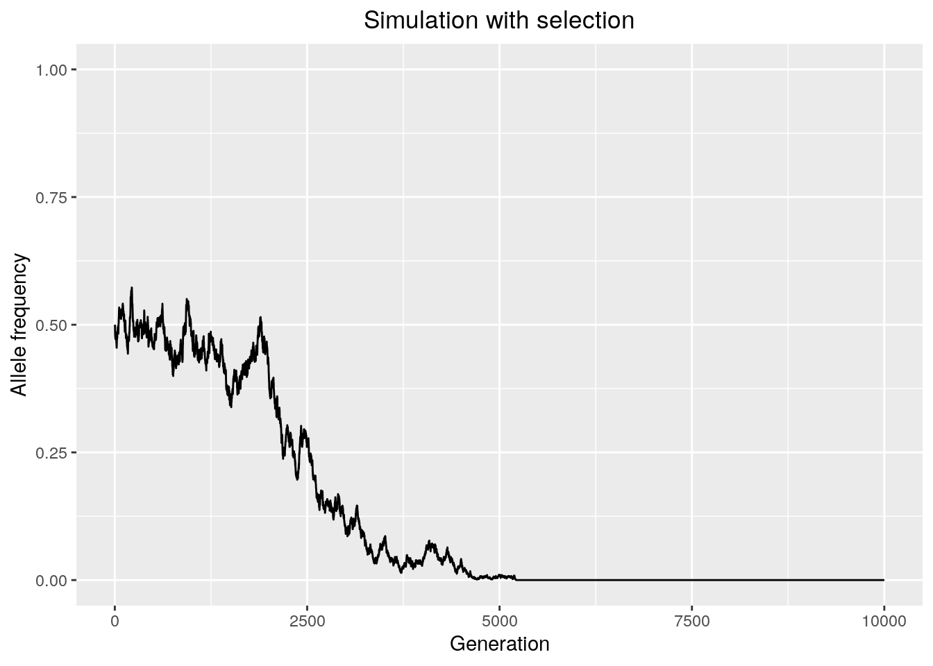

Run and plot the simulation without selection:

results <- run_sim_selection(Ne = 10000,
                             freq = 0.5,
                             generations = 10000,
                             s = 0)
ggplot() +
  geom_line(data = results, aes(x = gen, y = afs)) +
  ylim(0, 1) +
  ylab("Allele frequency") +
  xlab("Generation") +
  ggtitle("Simulation without selection") +
  theme(plot.title = element_text(hjust = 0.5)) # to center the title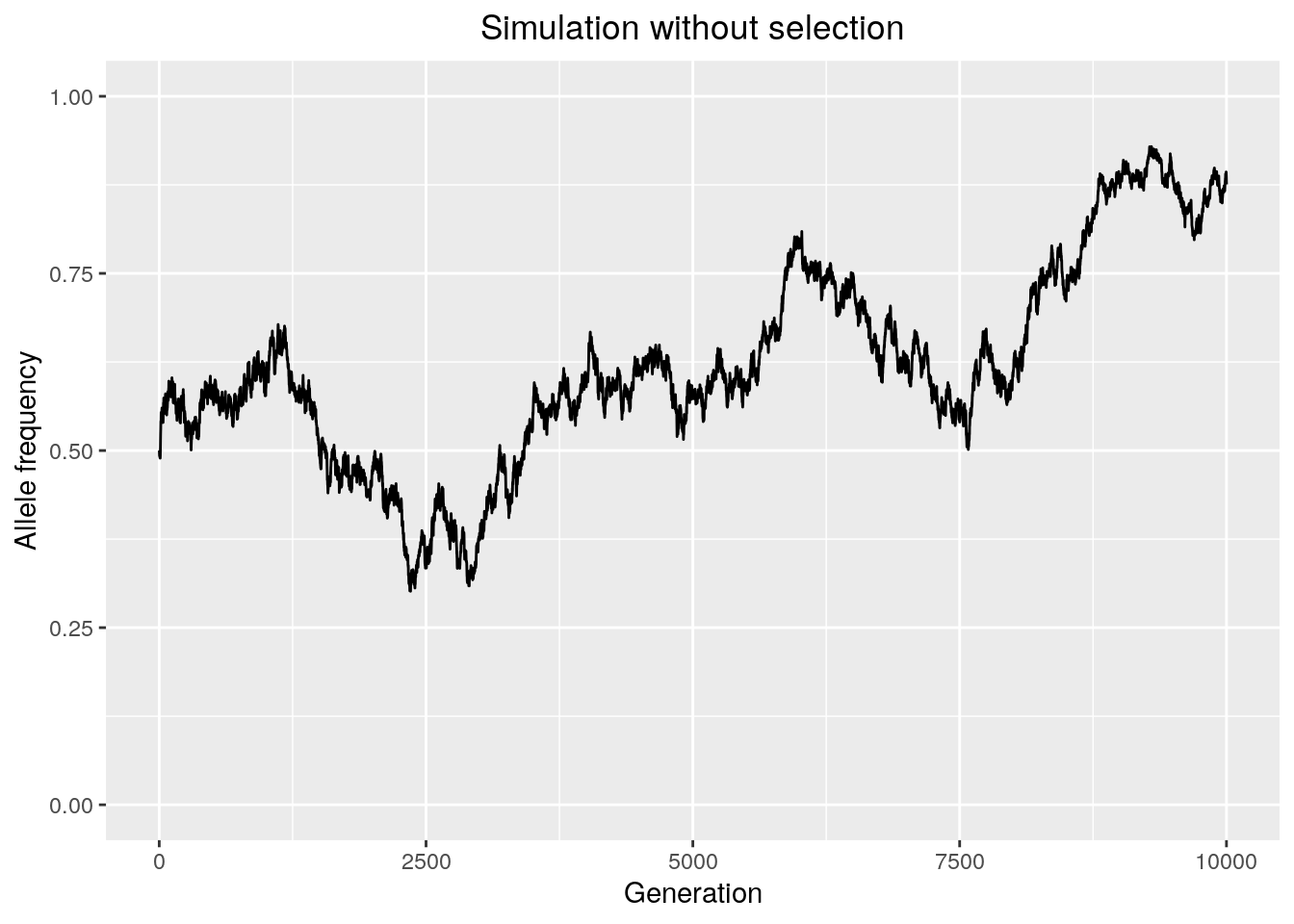

We observe that selection tends to decrease the time it takes for an allele to either fix or go extinct, because it directionally biases the probability of sampling that allele. Decreasing the absolute value of the selection coefficient will make the simulation behave more like drift.