8.20 Homework

8.20.0.1 Learning Objectives

Interpret results of a GWAS
Practice manipulating tabular data

8.20.0.2 Assignment

Run a GWAS of \(\mathrm{IC_{50}}\) for the drug CB1908, using the same genotype data as before. The phenotypes are located in CB1908_IC50.txt.

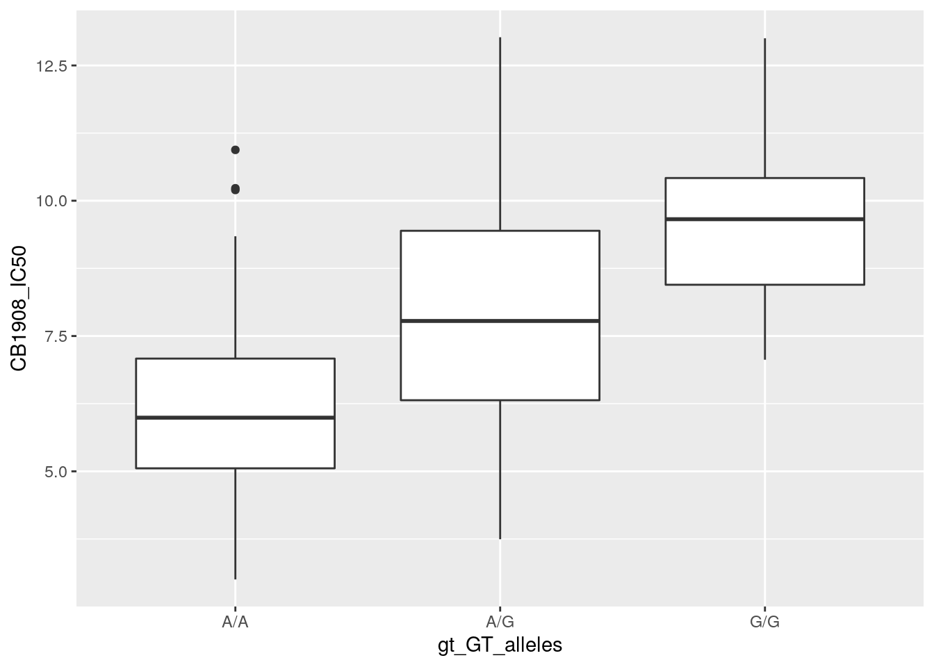
Make a QQ plot and a Manhattan plot of your results. Do you have any genome-wide significant hits? Are they located in or near a gene? For the top GWAS hit, plot the phenotype stratified by genotype. (Use top_snp_hw.vcf to get the genotypes of the top hit.)

Solution

# perform association test with PLINK
system(command = "./plink --file genotypes --linear --allow-no-sex --pheno CB1908_IC50.txt --pheno-name CB1908_IC50")

# read in gwas results
results <- read.table(file = "plink.assoc.linear", header = TRUE) %>%
  mutate(index = row_number()) %>%
  arrange(P)

# qq plot
qq(results$P)

# manhattan plot
manhattan(results)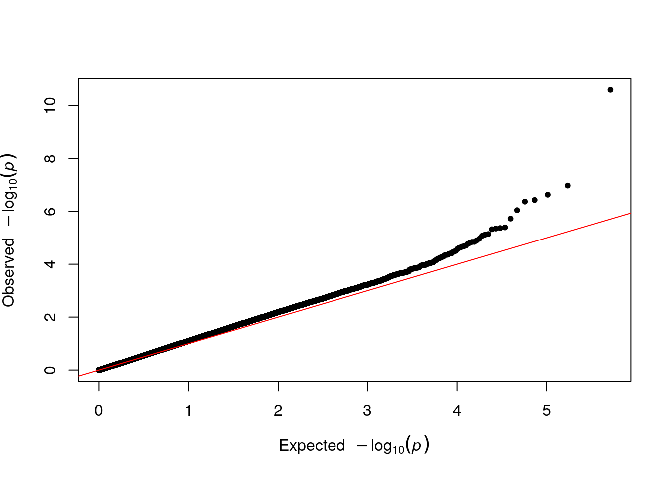

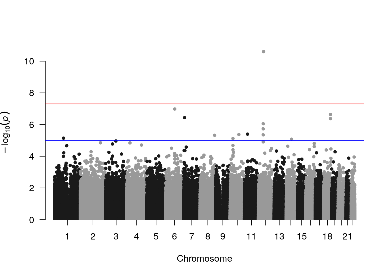
On the Manhattan plot, there’s one hit that reaches genome-wide significance.

# view top GWAS hit
results[1, ]

##   CHR        SNP       BP A1 TEST NMISS  BETA STAT         P
## 1  12 rs10876043 49190411  G  ADD   161 1.779 7.18 2.518e-11

From looking it up in the UCSC Genome Browser, rs10876043 lies within an intron of the DIP2B gene. Finally, we plot this SNP’s genotype stratified by phenotype, using top_snp_hw.vcf.

# extract top SNP and convert to tidy df
top_snp <- vcfR2tidy(read.vcfR("top_snp_hw.vcf"))

## Scanning file to determine attributes.
## File attributes:
##   meta lines: 27
##   header_line: 28
##   variant count: 1
##   column count: 185
## 
Meta line 27 read in.
## All meta lines processed.
## gt matrix initialized.
## Character matrix gt created.
##   Character matrix gt rows: 1
##   Character matrix gt cols: 185
##   skip: 0
##   nrows: 1
##   row_num: 0
## 
Processed variant: 1
## All variants processed

## Extracting gt element GT

# get genotype dataframe
top_snp_gt <- top_snp$gt %>%
  drop_na()

# read in phenotype dataframe
phenotypes <- read.table("CB1908_IC50.txt", header = TRUE)

# merge genotype and phenotype info
gwas_data <- merge(top_snp_gt, phenotypes,
                   by.x = "Indiv", by.y = "IID")

# plot genotype by phenotype boxplots
ggplot(data = gwas_data) +
  geom_boxplot(aes(x = gt_GT_alleles,
                   y = CB1908_IC50))

## Warning: Removed 2 rows containing non-finite values (stat_boxplot).