7.3 Multiple testing

What are statistical challenges of performing a test multiple times?

When we perform any test multiple times, we increase the risk that a “significant” result is only significant by chance.

Under the null hypothesis, we assume that p-values follow a uniform distribution (i.e., a flat distribution from 0 to 1). We can plot this null distribution in R:

# generate 1,000,000 "p-values" from a uniform distribution
pvalues <- runif(1000000)
# histogram with R's base plotting function
hist(pvalues)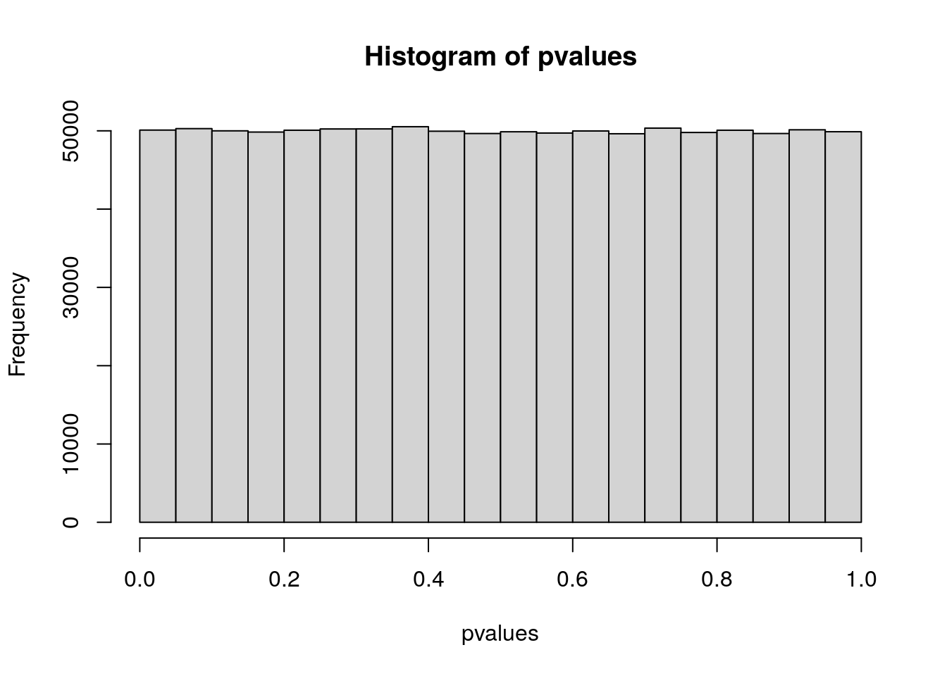

If we use the typical p-value threshold of \(0.05\), 5% of our tests will have \(p < 0.05\), even though these p-values were simulated from a null distribution (i.e., no real association).

How do we correct for multiple testing?

One common multiple testing correction method, Bonferroni correction, sets a stricter p-value threshold. With Bonferroni, you divide your desired p-value by the number of independent tests you conducted.

Are GWAS tests (variants) statistically independent? How does this affect our p-value threshold?

As we learned in the LD module, the genotypes of nearby variants are correlated.

This non-independence means that we can be less strict with multiple testing correction, because we aren’t performing as many independent tests as we think we are.

Researchers have calculated that \(\mathbf{5*10^{-8}}\) is an appropriate p-value threshold for GWAS in humans, given the amount of LD in human genomes.