8.9 Phenotype data

Our phenotype for this GWAS is the \(\mathbf{IC_{50}}\) – the concentration of the GS451 drug that at which we observe 50% viability in cell culture.

# read in phenotypes
phenotypes <- read.table("GS451_IC50.txt", header = TRUE)

head(phenotypes)

##    FID  IID GS451_IC50
## 1 1001 1001   5.594256
## 2 1002 1002   8.525633
## 3 1003 1003  12.736739
## 4 1004 1004  12.175201
## 5 1005 1005   9.936742
## 6 1006 1006   9.163483

The columns of this table are:

FID & IID: Family and individual IDs of the individual
GS451_IC50: Measured \(\mathrm{IC_{50}}\) for the drug of interest

Plot the distribution of the phenotype.

ggplot(data = phenotypes,
       aes(x = GS451_IC50)) +
  geom_histogram()

## `stat_bin()` using `bins = 30`. Pick better value with `binwidth`.

## Warning: Removed 1 rows containing non-finite values (stat_bin).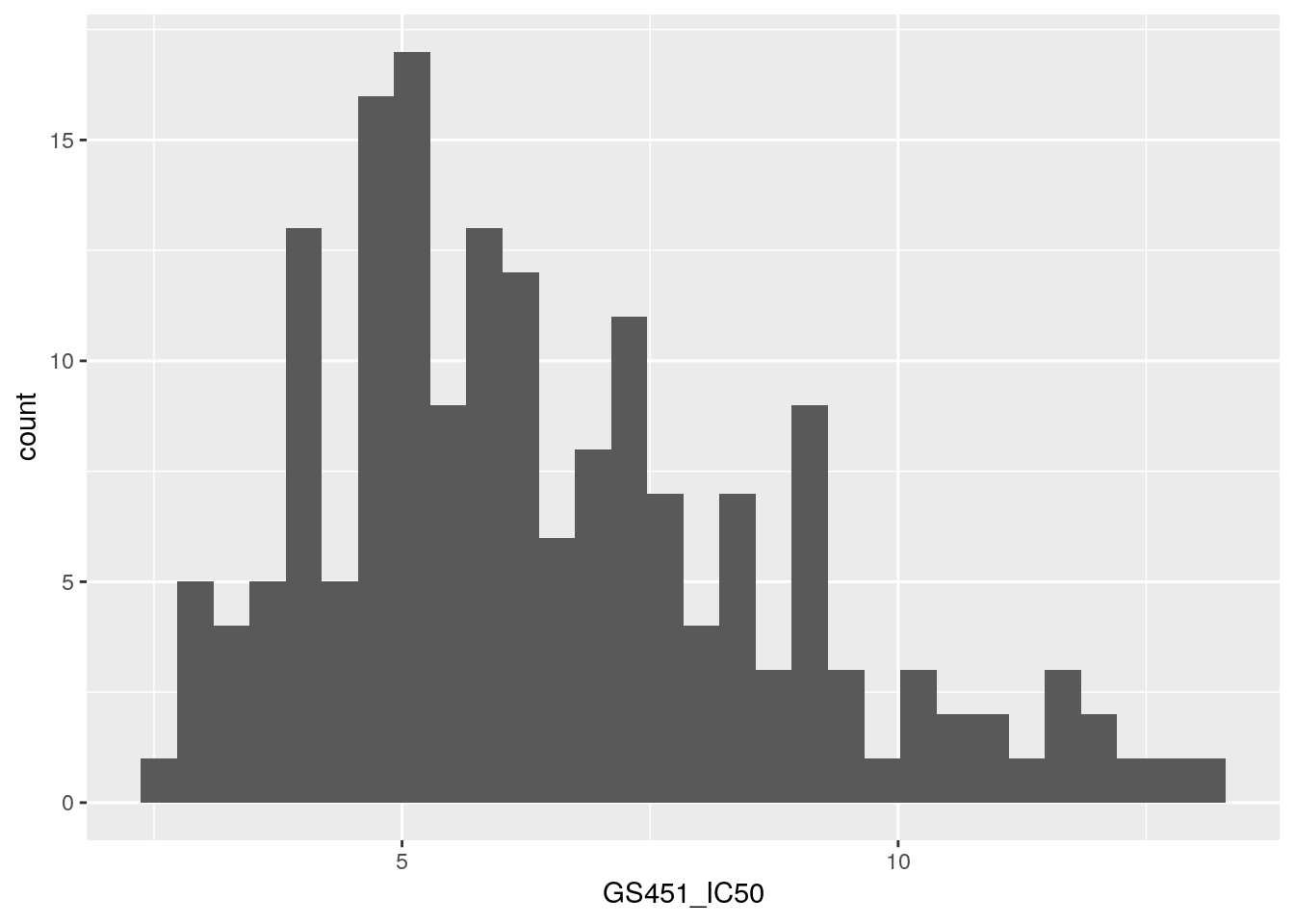

This data looks approximately normally distributed. This is important to check because this is one of the assumptions of linear regression, which we’ll be using to perform the GWAS.