8.18 Top GWAS SNP

One common future direction for GWAS studies is following up on the top SNP(s). Read in top_snp.vcf, a VCF of just the top SNP in the dataset, so that we can plot boxplots of the top SNP genotype stratified by phenotype:

# extract genotypes of the top SNP
top_snp <- vcfR2tidy(read.vcfR("top_snp.vcf"))

## Scanning file to determine attributes.
## File attributes:
##   meta lines: 27
##   header_line: 28
##   variant count: 1
##   column count: 185
## 
Meta line 27 read in.
## All meta lines processed.
## gt matrix initialized.
## Character matrix gt created.
##   Character matrix gt rows: 1
##   Character matrix gt cols: 185
##   skip: 0
##   nrows: 1
##   row_num: 0
## 
Processed variant: 1
## All variants processed

## Extracting gt element GT

top_snp_gt <- top_snp$gt %>%
  drop_na()

# merge with phenotype data
gwas_data <- merge(top_snp_gt, phenotypes,
                   by.x = "Indiv", by.y = "IID")

# plot boxplots
ggplot(data = gwas_data) +
  geom_boxplot(aes(x = gt_GT_alleles,
                   y = GS451_IC50))

## Warning: Removed 1 rows containing non-finite values (stat_boxplot).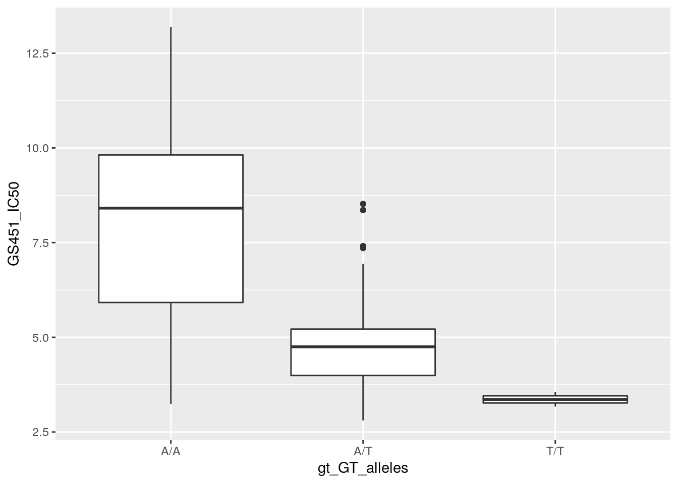

Other potential follow-up directions include:

Investigating the genomic environment in the UCSC Genome Browser
Looking at nearby haplotype structure with LDproxy
- Note that the genotype data we’re using come from the Yoruba population
Using the Geography of Genetic Variants browser to find the global allele frequencies of the variant
Search for SNP in a phenotype database to see if there are other associations with it