4.11 LDlink

LDlink is a web application that allows you to compute and visualize linkage disequilibrium using data from the 1000 Genomes Project (the same dataset we’ve been using for this module).

Go to LDlink’s LDpair tool, which computes \(D'\) and \(r^2\) between pairs of SNPs. Using either the rsIDs or the chromosome and position of the two SNPs we looked at today, check our calculations for \(D'\) and \(r^2\). Make sure you:

Select All Populations, since we didn’t subset our data by population.
If using SNP position, note that our data was aligned to the GRCh38 reference genome.

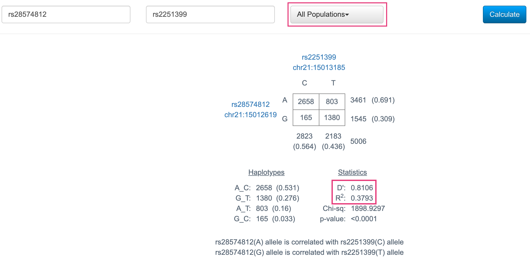
Fig. 5. LDpair results for the two SNPs from this class.

We can see that these \(D'\) and \(r^2\) statistics, as well as the 4x4 table, are very similar to what we calculated by hand! (The values aren’t identical because we’re using a slightly different genotyping dataset.)